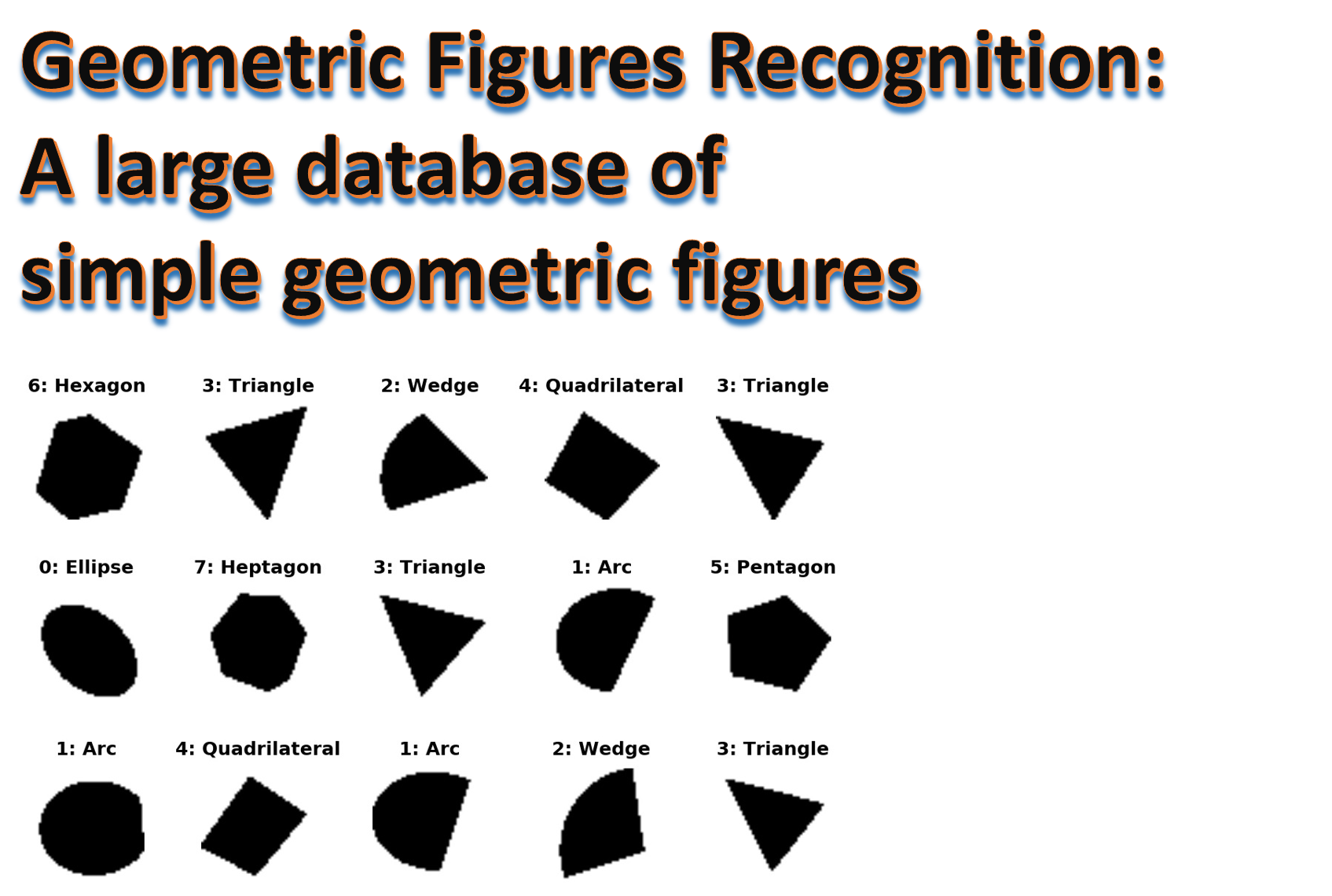
Geofig is a large data set of simple 48x48 pixels black and white geometrical shapes. It consists of 8 shape types:

0: Ellipse
1: Arc
2: Wedge
3: Triangle
4: Quadrilateral
5: Pentagon
6: Hexagon
7: Heptagon

They were generated by an automatic Python script with randomization on shapes. It was designed to be as simple as possible in order to serve as a first clean example for deep learning courses, introductory tutorials, and first course projects. We used grayscale 48x48 pixels images, so that it can be processed by standard pc systems with modest computing resources.

It is also intended to serve as a clear and simple minded data set for benchmarking deep learning libraries and deep learning hardware (like GPU systems). As far as we tried within the Keras library, achieving high accuracy prediction scores does require a non-trivial effort and compute time. So it does make a good challenge for tutorials and course projects for image recognition.

The GeoFig data set consists of 4 HDF5 files, each contains 80,000 48x48 pixels black/white images. So in total, we have 320,000 48x48 black/white images. We believe that 20K images are enough for training, so you may need to download only the first set. But in case you need more images, you have 300K more to choose from. All the data sets are balanced. That is they contain equal numbers of shapes from each group. And of course, there are no duplications! All the 320K images are unique.

  1. http://www.samyzaf.com/ML/geofig/geofig1.h5.zip
  2. http://www.samyzaf.com/ML/geofig/geofig2.h5.zip
  3. http://www.samyzaf.com/ML/geofig/geofig3.h5.zip
  4. http://www.samyzaf.com/ML/geofig/geofig4.h5.zip

You will need to install the h5py Python module. Reading and writing HDF5 files can be easily learned from the following tutorial: https://www.getdatajoy.com/learn/Read_and_Write_HDF5_from_Python

Prerequisites

The code for this IPython notebook was tested on Windows 10, Python 2.7 with keras, numpy, matplotlib and jupyter. The deep learning hardware we used was an NVIDIA GPU (GeForce/GTX950) with cuDNN version 5103. Of course, it can also be run on a traditional CPU but it will be significantly slower (not recommended!).

To run the code in this notebook, you will need to download a few course libraries which we use in other examples of this course. They can be downloaded in one zip file from my Github repository:
https://github.com/samyzaf/kerutils

You can also view and download each file individually:

  1. http://www.samyzaf.com/cgi-bin/view_file.py?file=ML/lib/kerutils.py
  2. http://www.samyzaf.com/cgi-bin/view_file.py?file=ML/lib/dlutils.py
  3. http://www.samyzaf.com/cgi-bin/view_file.py?file=ML/lib/imgutils.py
  4. http://www.samyzaf.com/cgi-bin/view_file.py?file=ML/lib/progmeter.py
  5. http://www.samyzaf.com/cgi-bin/view_file.py?file=ML/style-notebook.css (notebook stylesheet)

Here are the Python modules and basic definitions we need for an example of how to use the GeoFig data set

In [1]:
from keras.datasets import cifar10
from keras.preprocessing.image import ImageDataGenerator
from keras.models import Sequential, load_model
from keras.layers import Dense, Dropout, Activation, Flatten
from keras.layers import Convolution2D, MaxPooling2D, AveragePooling2D, ZeroPadding2D
from keras.optimizers import SGD
from keras.constraints import maxnorm
from keras.utils import np_utils
from keras.layers.advanced_activations import SReLU, ELU, LeakyReLU
from keras.utils.visualize_util import plot
from keras.layers.noise import GaussianNoise
import matplotlib.pyplot as plt
import matplotlib.cm
from matplotlib import rcParams
from kerutils import *
from imgutils import *
%matplotlib inline

class_name = {
    0: 'Ellipse',
    1: 'Arc',
    2: 'Wedge',
    3: 'Triangle',
    4: 'Quadrilateral',
    5: 'Pentagon',
    6: 'Hexagon',
    7: 'Heptagon',
}

nb_classes = len(class_name)   # Number of features
classes = range(nb_classes)    # List of features (as integers)
Using Theano backend.
DEBUG: nvcc STDOUT mod.cu
   Creating library C:/Users/samy/AppData/Local/Theano/compiledir_Windows-10-10.0.14393-Intel64_Family_6_Model_94_Stepping_3_GenuineIntel-2.7.11-64/tmpikjdfc/265abc51f7c376c224983485238ff1a5.lib and object C:/Users/samy/AppData/Local/Theano/compiledir_Windows-10-10.0.14393-Intel64_Family_6_Model_94_Stepping_3_GenuineIntel-2.7.11-64/tmpikjdfc/265abc51f7c376c224983485238ff1a5.exp

Using gpu device 0: GeForce GTX 950 (CNMeM is enabled with initial size: 80.0% of memory, cuDNN 5103)
c:\anaconda2\lib\site-packages\theano\sandbox\cuda\__init__.py:600: UserWarning: Your cuDNN version is more recent than the one Theano officially supports. If you see any problems, try updating Theano or downgrading cuDNN to version 5.
  warnings.warn(warn)
In [1]:
# These are css/html styles for good looking ipython notebooks
from IPython.core.display import HTML
css = open('style-notebook.css').read()
HTML('<style>{}</style>'.format(css));

Preparing training and validation data sets

The archived data sets above are too large for early experimentation, so we suggest that you start with a smaller data sets first, and later increase their size if needed.

The imgutils module (see above) contains several utilities for manipulating HDF5 files. The function save_h5_from_file can be used to extract a subset of images to an HDF5 file from a larger HDF5. It accepts three arguments:

  1. source HDF5 pool of images
  2. target HDF5 file (for saving the subset)
  3. Class size: how many images in each shape class. We have 8 shape classes, so the total number of shapes in the subset file should be 8 times larger.
In [3]:
save_h5_from_file("geofig1.h5", "train.h5", 1000)
save_h5_from_file("geofig2.h5", "test.h5", 200)
Total num images in file: 80000
Load progress: 100%   
Time: 26.52 seconds
Writing file: train.h5
Progress: 100%   
Time: 3.83 seconds
Total num images in file: 80000
Load progress: 100%   
Time: 27.18 seconds
Writing file: test.h5
Progress: 100%   
Time: 0.90 seconds
Out[3]:
'test.h5'

Note that we made sure the training and validation data are disjoint (no common images) by extracting the from two different pools.

Load training and test data

The imgutils module also contains a utility load_data for loading HDF5 files to memory (as Numpy arrays). This method accepts the names of your training and validation data set files, and it returns the following six Numpy arrays:

  1. X_train: an array of 8000 images whose shape is 8000x48x48.
  2. y_train: a one dimensional array of 8000 integers representing the class of each image in X_train.
  3. Y_train: an 8000 array of one-hot vectors needed for Keras model. For more details see: http://stackoverflow.com/questions/29831489/numpy-1-hot-array
  4. X_test: an array of 1000 validation images (1000x48x48)
  5. y_test: validation class array
  6. Y_test: one-hot vectors for the validation samples

It should be noted that in additional to reading the images from the HDF5 file, the load_data method also performs some normalization of the image data like scaling it to a unit interval and centering it around the mean value. You can control these actions by additional optional options of this command. Please look at the source code to learn more.

In [4]:
X_train, y_train, Y_train, X_test, y_test, Y_test = load_data('train.h5', 'test.h5')

print('X_train shape:', X_train.shape)
print(X_train.shape[0], 'training samples')
print(X_test.shape[0], 'validation samples')
Loading training data set: train.h5
Total num images in file: 8000
Load progress: 100%   
Time: 3.13 seconds
Loading validation data set: test.h5
Total num images in file: 1600
Load progress: 100%   
Time: 0.79 seconds
8000 training samples
1600 validation samples
Image shape: (48L, 48L, 1L)
X_train shape: (8000L, 48L, 48L, 1L)
8000 training samples
1600 validation samples

Let's also write two small utilities for drawing samples of images, so we can inspect our results visually.

In [23]:
def draw_image(img, id):
    img = img.reshape(48,48)
    plt.imshow(img, cmap='gray', interpolation='none')
    plt.title("%d: %s" % (id, class_name[id]), fontsize=15, fontweight='bold', y=1.08)
    plt.axis('off')
    plt.show()

Let's draw image 18 in the X_train array as example

In [24]:
draw_image(X_train[18], y_train[18])

As we can see, the image is a bit blurry due to the normalization procedures that the load_data method has done to the original data. If you want to draw the raw data as it is in the HDF5 file, use the h5_get method to extract the raw image from the HDF5 file directly:

In [29]:
img = h5_get('train.h5', 'img_19') # images in h5 files are numbered from 1
id = y_train[18]
draw_image(img, id)

Sometimes we want to inspect a larger group of images in parallel, so we also provide a method for drawing a grid of consecutive images.

In [41]:
def draw_sample(X, y, n, rows=4, cols=4, imfile=None, fontsize=9):
    for i in range(0, rows*cols):
        plt.subplot(rows, cols, i+1)
        img = X[n+i].reshape(48,48)
        plt.imshow(img, cmap='gray', interpolation='none')
        id = y[n+i]
        plt.title("%d: %s" % (id, class_name[id]), fontsize=fontsize, y=1.08)
        plt.axis('off')
        plt.subplots_adjust(wspace=0.8, hspace=0.1)
In [42]:
draw_sample(X_train, y_train, 400, 3, 5)

Building A Neural Network for GeoFig

We will start with a simple Keras model which combines one Convolution2D layer with two Dense layers. Although simple in terms of code, it is too expensive in terms of computation and hardware, as it contains 70 million parameters! This is way too much and should be avoided in general. However, we want to experiment with the common use of Dense layers and see why they are not good for image processing. In general, Dense layers should be avoided as much as possible when dealing with image data. The general practice is to use Convolution and Pooling layers. These two types of layers are explained in more detail in the following two articles, which we recommend to read before you approach the following code:

  1. http://www.cs.toronto.edu/~kriz/learning-features-2009-TR.pdf
  2. http://cs231n.github.io/convolutional-networks/

Lets Train Model 1

We now define our first model for the recognizing GeoFig shapes. Note that unlike the common practice, we decided to use the SReLU activation method instead of the more popular relu activation. We did several test with relu but SReLU seems to be more appropriate for GeoFig. One of the amazing facts about SReLU is that it adapts itself during the learning process and not a constant function as other activations. You may read more about it in the following papers:

  1. https://arxiv.org/abs/1512.07030
  2. https://arxiv.org/pdf/1512.07030.pdf
In [73]:
nb_epoch = 100
batch_size = 32
input_shape = X_train.shape[1:]

model = Sequential(name="model_1")
model.add(Convolution2D(64, 3, 3, input_shape=input_shape))
model.add(SReLU())

model.add(Flatten())

model.add(Dense(512))
model.add(SReLU())
model.add(Dropout(0.4))

model.add(Dense(256))
model.add(SReLU())
model.add(Dropout(0.4))

model.add(Dense(nb_classes))
model.add(Activation('softmax'))

print(model.summary())
save_model_summary(model, "model_1_summary.txt")
write_file("model_1.json", model.to_json())
fmon = FitMonitor(thresh=0.09, minacc=0.999, filename="model_1_autosave.h5")

model.compile(optimizer='adam', loss='categorical_crossentropy', metrics=['accuracy'])

hist = model.fit(
    X_train,
    Y_train,
    batch_size=batch_size,
    nb_epoch=nb_epoch,
    shuffle=True,
    validation_data=(X_test, Y_test),
    verbose=0,
    callbacks = [fmon]
)

model_file = "model_1.h5"
print("Saving model to:", model_file)
model.save(model_file)
plot(model, to_file="model_1_scheme.png", show_layer_names=False, show_shapes=True)

show_scores(model, hist, X_train, Y_train, X_test, Y_test)
____________________________________________________________________________________________________
Layer (type)                     Output Shape          Param #     Connected to                     
====================================================================================================
convolution2d_7 (Convolution2D)  (None, 46L, 46L, 64)  640         convolution2d_input_4[0][0]      
____________________________________________________________________________________________________
srelu_13 (SReLU)                 (None, 46L, 46L, 64)  541696      convolution2d_7[0][0]            
____________________________________________________________________________________________________
flatten_4 (Flatten)              (None, 135424)        0           srelu_13[0][0]                   
____________________________________________________________________________________________________
dense_10 (Dense)                 (None, 512)           69337600    flatten_4[0][0]                  
____________________________________________________________________________________________________
srelu_14 (SReLU)                 (None, 512)           2048        dense_10[0][0]                   
____________________________________________________________________________________________________
dropout_7 (Dropout)              (None, 512)           0           srelu_14[0][0]                   
____________________________________________________________________________________________________
dense_11 (Dense)                 (None, 256)           131328      dropout_7[0][0]                  
____________________________________________________________________________________________________
srelu_15 (SReLU)                 (None, 256)           1024        dense_11[0][0]                   
____________________________________________________________________________________________________
dropout_8 (Dropout)              (None, 256)           0           srelu_15[0][0]                   
____________________________________________________________________________________________________
dense_12 (Dense)                 (None, 8)             2056        dropout_8[0][0]                  
____________________________________________________________________________________________________
activation_4 (Activation)        (None, 8)             0           dense_12[0][0]                   
====================================================================================================
Total params: 70,016,392
Trainable params: 70,016,392
Non-trainable params: 0
____________________________________________________________________________________________________
None
Train begin: 2016-12-29 02:33:40
Stop file: stop_training_file.keras (create this file to stop training gracefully)
Pause file: pause_training_file.keras (create this file to pause training and view graphs)
batch_size = 32
do_validation = True
metrics = ['loss', 'acc', 'val_loss', 'val_acc']
nb_epoch = 100
nb_sample = 8000
verbose = 0
.....05% epoch=5, acc=0.913500, loss=0.237724, val_acc=0.875625, val_loss=0.400973, time=0.043 hours
.....10% epoch=10, acc=0.937750, loss=0.179296, val_acc=0.888125, val_loss=0.479060, time=0.085 hours
.....15% epoch=15, acc=0.960625, loss=0.123028, val_acc=0.894375, val_loss=0.547391, time=0.127 hours
.....20% epoch=20, acc=0.963500, loss=0.127408, val_acc=0.870625, val_loss=0.655237, time=0.169 hours
.....25% epoch=25, acc=0.964500, loss=0.123090, val_acc=0.888125, val_loss=0.633842, time=0.211 hours
.....30% epoch=30, acc=0.976375, loss=0.083112, val_acc=0.902500, val_loss=0.571396, time=0.253 hours
.....35% epoch=35, acc=0.973500, loss=0.097881, val_acc=0.904375, val_loss=0.689928, time=0.295 hours
.....40% epoch=40, acc=0.982750, loss=0.068070, val_acc=0.900625, val_loss=0.642138, time=0.336 hours
.....45% epoch=45, acc=0.982625, loss=0.073193, val_acc=0.908750, val_loss=0.651504, time=0.378 hours
.....50% epoch=50, acc=0.981375, loss=0.080499, val_acc=0.915000, val_loss=0.670766, time=0.420 hours
.....55% epoch=55, acc=0.978250, loss=0.095815, val_acc=0.915625, val_loss=0.656580, time=0.462 hours
.....60% epoch=60, acc=0.979750, loss=0.078105, val_acc=0.903125, val_loss=0.769453, time=0.504 hours
.....65% epoch=65, acc=0.986875, loss=0.053917, val_acc=0.910625, val_loss=0.646367, time=0.545 hours
.....70% epoch=70, acc=0.980500, loss=0.092110, val_acc=0.891250, val_loss=0.819553, time=0.587 hours
.....75% epoch=75, acc=0.984750, loss=0.078778, val_acc=0.913125, val_loss=0.801312, time=0.629 hours
.....80% epoch=80, acc=0.989250, loss=0.046153, val_acc=0.908750, val_loss=0.792932, time=0.671 hours
.....85% epoch=85, acc=0.988750, loss=0.051939, val_acc=0.912500, val_loss=0.780656, time=0.713 hours
.....90% epoch=90, acc=0.985875, loss=0.079065, val_acc=0.908750, val_loss=0.815327, time=0.755 hours
.....95% epoch=95, acc=0.988500, loss=0.064978, val_acc=0.908125, val_loss=0.892710, time=0.797 hours
.... 99% epoch=99 acc=0.985500 loss=0.077015
Train end: 2016-12-29 03:23:30
Total run time: 0.830 hours
max_acc = 0.989750  epoch = 81
max_val_acc = 0.925000  epoch = 79
No checkpoint model found.
Saving model to: model_1.h5
Training: accuracy   = 0.998500 loss = 0.009213
Validation: accuracy = 0.895625 loss = 1.100054
Over fitting score   = 0.074623
Under fitting score  = 0.070641
Params count: 70016392
stop epoch = 99
nb_epoch = 100
batch_size = 32
nb_sample = 8000
In [74]:
loss, accuracy = model.evaluate(X_train, Y_train, verbose=0)
print("Training: accuracy = %f  ;  loss = %f" % (accuracy, loss))
Training: accuracy = 0.998500  ;  loss = 0.009213
In [75]:
loss, accuracy = model.evaluate(X_test, Y_test, verbose=0)
print("Validation: accuracy1 = %f  ;  loss1 = %f" % (accuracy, loss))
Validation: accuracy1 = 0.895625  ;  loss1 = 1.100054

Although the training accuracy is quite high (99.82% !), the overall result is not good. The 10% gap with the validation accuracy is an indication of overfitting (which is also clearly noticeable from the accuracy and loss graphs above). Our model is successful on the training set only and is no as successful for any other data.

Inspecting the output

Befor we search for a new model, let's take a quick look on some of the cases that our model missed. It may give us clues on the strengths and weaknesses of NN models, and what we can expect from these artificial models.

The predict_classes method is helpful for getting a vector (y_pred) of the predicted classes of model1. We should compare y_pred to the expected true classes y_test in order to get the false cases:

In [47]:
y_pred = model.predict_classes(X_test)
1600/1600 [==============================] - 0s     
In [49]:
true_preds = [(x,y) for (x,y,p) in zip(X_test, y_test, y_pred) if y == p]
false_preds = [(x,y,p) for (x,y,p) in zip(X_test, y_test, y_pred) if y != p]
print("Number of valid predictions: ", len(true_preds))
print("Number of invalid predictions:", len(false_preds))
Number of valid predictions:  1437
Number of invalid predictions: 163

The array false_preds consists of all triples (x,y,p) where x is an image, y is its true class, and p is the false predicted value of model.

Lets visualize a sample of 15 items:

In [58]:
for i,(x,y,p) in enumerate(false_preds[0:15]):
    plt.subplot(3, 5, i+1)
    img = x.reshape(48,48)
    plt.imshow(img, cmap='gray')
    plt.title("%d\ny: %s\np: %s" % (i, class_name[y], class_name[p]), fontsize=9, loc='left')
    plt.axis('off')
    plt.subplots_adjust(wspace=0.8, hspace=0.6)

We see that our model sometimes confuses between a Wedge and an Arc in case that the Wedge angle is close to $180^\circ$ degrees. We see this in examples 3, 8, and possibly 4 (although in example 4 the angle is not so close to $180^\circ$). Sometimes when the Arc angle is very small, the model thinks it's an ellipse (like in examples 0 and 13). The confusion between a Heptagon and a Hexagon can also be understood likewise, but in all other cases there is no such explanation for the model error. Obviously we need to work harder for a better model. Could be that our training set is too small (only 8000 samples) but most probably we need to use more convolution layers.

Second Keras Model for GeoFig database

Lets try to add an additional Convolution2D layer and reduce the width of the Dense layers. The number of parameters is still too high (32 millions), but much less than model 1.

In [59]:
nb_epoch = 100
batch_size = 32
input_shape = X_train.shape[1:]

model = Sequential(name="model_2")
model.add(Convolution2D(64, 3, 3, input_shape=input_shape))
model.add(SReLU())

model.add(Convolution2D(64, 3, 3, input_shape=input_shape))
model.add(SReLU())

model.add(Flatten())

model.add(Dense(256))
model.add(SReLU())
model.add(Dropout(0.4))

model.add(Dense(64))
model.add(SReLU())
model.add(Dropout(0.4))

model.add(Dense(nb_classes))
model.add(Activation('softmax'))

print(model.summary())
save_model_summary(model, "model_2_summary.txt")
write_file("model_2.json", model.to_json())
fmon = FitMonitor(thresh=0.09, minacc=0.999, filename="model_2_autosave.h5")

model.compile(optimizer='adam', loss='categorical_crossentropy', metrics=['accuracy'])

hist = model.fit(
    X_train,
    Y_train,
    batch_size=batch_size,
    nb_epoch=nb_epoch,
    shuffle=True,
    validation_data=(X_test, Y_test),
    verbose=0,
    callbacks = [fmon]
)

model_file = "model_2.h5"
print("Saving model to:", model_file)
model.save(model_file)
plot(model, to_file="model_2_scheme.png", show_layer_names=False, show_shapes=True)

show_scores(model, hist, X_train, Y_train, X_test, Y_test)
____________________________________________________________________________________________________
Layer (type)                     Output Shape          Param #     Connected to                     
====================================================================================================
convolution2d_2 (Convolution2D)  (None, 46L, 46L, 64)  640         convolution2d_input_2[0][0]      
____________________________________________________________________________________________________
srelu_4 (SReLU)                  (None, 46L, 46L, 64)  541696      convolution2d_2[0][0]            
____________________________________________________________________________________________________
convolution2d_3 (Convolution2D)  (None, 44L, 44L, 64)  36928       srelu_4[0][0]                    
____________________________________________________________________________________________________
srelu_5 (SReLU)                  (None, 44L, 44L, 64)  495616      convolution2d_3[0][0]            
____________________________________________________________________________________________________
flatten_2 (Flatten)              (None, 123904)        0           srelu_5[0][0]                    
____________________________________________________________________________________________________
dense_4 (Dense)                  (None, 256)           31719680    flatten_2[0][0]                  
____________________________________________________________________________________________________
srelu_6 (SReLU)                  (None, 256)           1024        dense_4[0][0]                    
____________________________________________________________________________________________________
dropout_3 (Dropout)              (None, 256)           0           srelu_6[0][0]                    
____________________________________________________________________________________________________
dense_5 (Dense)                  (None, 64)            16448       dropout_3[0][0]                  
____________________________________________________________________________________________________
srelu_7 (SReLU)                  (None, 64)            256         dense_5[0][0]                    
____________________________________________________________________________________________________
dropout_4 (Dropout)              (None, 64)            0           srelu_7[0][0]                    
____________________________________________________________________________________________________
dense_6 (Dense)                  (None, 8)             520         dropout_4[0][0]                  
____________________________________________________________________________________________________
activation_2 (Activation)        (None, 8)             0           dense_6[0][0]                    
====================================================================================================
Total params: 32,812,808
Trainable params: 32,812,808
Non-trainable params: 0
____________________________________________________________________________________________________
None
DEBUG: nvcc STDOUT mod.cu
   Creating library C:/Users/samy/AppData/Local/Theano/compiledir_Windows-10-10.0.14393-Intel64_Family_6_Model_94_Stepping_3_GenuineIntel-2.7.11-64/tmp8effip/2528e054188ee230779c451bef51f4a2.lib and object C:/Users/samy/AppData/Local/Theano/compiledir_Windows-10-10.0.14393-Intel64_Family_6_Model_94_Stepping_3_GenuineIntel-2.7.11-64/tmp8effip/2528e054188ee230779c451bef51f4a2.exp

Train begin: 2016-12-28 23:22:21
Stop file: stop_training_file.keras (create this file to stop training gracefully)
Pause file: pause_training_file.keras (create this file to pause training and view graphs)
batch_size = 32
do_validation = True
metrics = ['loss', 'acc', 'val_loss', 'val_acc']
nb_epoch = 100
nb_sample = 8000
verbose = 0
.....05% epoch=5, acc=0.911750, loss=0.251112, val_acc=0.916875, val_loss=0.258909, time=0.075 hours
.....10% epoch=10, acc=0.957625, loss=0.135432, val_acc=0.933750, val_loss=0.254242, time=0.138 hours
.....15% epoch=15, acc=0.970125, loss=0.092968, val_acc=0.936875, val_loss=0.277017, time=0.201 hours
.....20% epoch=20, acc=0.978750, loss=0.068480, val_acc=0.938125, val_loss=0.382742, time=0.263 hours
.....25% epoch=25, acc=0.983000, loss=0.066845, val_acc=0.932500, val_loss=0.506390, time=0.326 hours
.....30% epoch=30, acc=0.984500, loss=0.060035, val_acc=0.933750, val_loss=0.402247, time=0.389 hours
.....35% epoch=35, acc=0.984750, loss=0.048144, val_acc=0.939375, val_loss=0.420728, time=0.452 hours
.....40% epoch=40, acc=0.988625, loss=0.054338, val_acc=0.931250, val_loss=0.484559, time=0.515 hours
.....45% epoch=45, acc=0.988875, loss=0.046215, val_acc=0.943125, val_loss=0.405237, time=0.578 hours
.....50% epoch=50, acc=0.989125, loss=0.052696, val_acc=0.948125, val_loss=0.430331, time=0.641 hours
.....55% epoch=55, acc=0.988250, loss=0.052983, val_acc=0.936875, val_loss=0.519568, time=0.704 hours
.....60% epoch=60, acc=0.992500, loss=0.033509, val_acc=0.936250, val_loss=0.521191, time=0.768 hours
.....65% epoch=65, acc=0.993500, loss=0.031153, val_acc=0.939375, val_loss=0.487436, time=0.831 hours
.....70% epoch=70, acc=0.993625, loss=0.026806, val_acc=0.934375, val_loss=0.555589, time=0.894 hours
.....75% epoch=75, acc=0.995875, loss=0.023594, val_acc=0.931875, val_loss=0.592238, time=0.957 hours
.....80% epoch=80, acc=0.991625, loss=0.043948, val_acc=0.932500, val_loss=0.574965, time=1.019 hours
.....85% epoch=85, acc=0.994875, loss=0.030035, val_acc=0.936250, val_loss=0.588983, time=1.082 hours
.....90% epoch=90, acc=0.994375, loss=0.032126, val_acc=0.921250, val_loss=0.791659, time=1.144 hours
.....95% epoch=95, acc=0.991875, loss=0.041362, val_acc=0.925625, val_loss=0.697123, time=1.207 hours
.... 99% epoch=99 acc=0.994875 loss=0.030149
Train end: 2016-12-29 00:37:48
Total run time: 1.258 hours
max_acc = 0.997125  epoch = 89
max_val_acc = 0.948125  epoch = 50
No checkpoint model found.
Saving model to: model_1.h5
Training: accuracy   = 0.999500 loss = 0.005213
Validation: accuracy = 0.935625 loss = 0.662881
Over fitting score   = 0.054801
Under fitting score  = 0.051126
Params count: 32812808
stop epoch = 99
nb_epoch = 100
batch_size = 32
nb_sample = 8000

Seems like the second Convolution layer that we added has reduced overfitting by almost 4%, but this is not good enough yet. The clear gap between the training and validation loss graph indicates that there's more room for improvement.

Validation credibility

Before proceeding to our third model, let's take a moment for discussing one more isue. From the two models above, we learn that training accuracy can be quite high (99.82% in model 1, and 99.95% in model 2), but we should not be impressed as we fall short in our validation sets. In some cases however we might be satisfied with what we got but would like to carry out further tests to make sure that the validation accuracy we have is not volatile. After all our validation set ("test.h5") has only 1600 samples, which might not be enough to trust in general.

Our imgutils contains a special method check_data_set for testing our model on as many samples as we wish from our large repository of samples (320K samples!). This method accepts three arguments:

  1. Keras model object
  2. HDF5 file of GeoFig images
  3. Number of images to sample

You may want to sample a few thousand images from each repository in order to gain confidence in your model. here are two examples of using this method which show that the validation accuracy we got is trustable:

In [63]:
check_data_set(model, "geofig4.h5", sample=5000)
Total num images in file: 80000
Sampling 5000 images from 80000
Load progress: 100%   
Time: 2.23 seconds
Loaded 5000 images
4992/5000 [============================>.] - ETA: 0sData shape: (5000L, 48L, 48L, 1L)
accuracy   = 0.935200 loss = 0.670067
Out[63]:
(0.93520000000000003, 0.67006727098466923)
In [64]:
check_data_set(model, "geofig3.h5", sample=10000)
Total num images in file: 80000
Sampling 10000 images from 80000
Load progress: 100%   
Time: 4.22 seconds
Loaded 10000 images
10000/10000 [==============================] - 7s     
Data shape: (10000L, 48L, 48L, 1L)
accuracy   = 0.936500 loss = 0.650812
Out[64]:
(0.9365, 0.65081230111322153)

Model 3

We will add a third Convolution layer, and increase the filter size to 5x5 in the first two layers. In adition, we add three new MaxPooling2D layers (one after each Convolution2D). The immediate effect of these layers is a drastic reduction in the model number of parameters from 90 million to 915K almost 1% of the size of model 1. Even if we get similar results to model 1, it would be considered a success and a proof for why Convolution and Pooling layers are the right kind of layers to use for image data.

In [65]:
nb_epoch = 100
batch_size = 32
input_shape = X_train.shape[1:]

model = Sequential(name="model_3")
model.add(Convolution2D(64, 5, 5, input_shape=input_shape))
model.add(SReLU())

model.add(MaxPooling2D(pool_size=(2, 2)))

model.add(Convolution2D(64, 5, 5, input_shape=input_shape))
model.add(SReLU())

model.add(MaxPooling2D(pool_size=(2, 2)))

model.add(Convolution2D(64, 3, 3, input_shape=input_shape))
model.add(SReLU())

model.add(MaxPooling2D(pool_size=(2, 2)))

model.add(Flatten())

model.add(Dense(256))
model.add(SReLU())
model.add(Dropout(0.5))

model.add(Dense(128))
model.add(SReLU())
model.add(Dropout(0.5))

model.add(Dense(nb_classes))
model.add(Activation('softmax'))

print(model.summary())
save_model_summary(model, "model_3_summary.txt")
write_file("model_3.json", model.to_json())
fmon = FitMonitor(thresh=0.09, minacc=0.999, filename="model_3_autosave.h5")

model.compile(optimizer='adam', loss='categorical_crossentropy', metrics=['accuracy'])

hist = model.fit(
    X_train,
    Y_train,
    batch_size=batch_size,
    nb_epoch=nb_epoch,
    shuffle=True,
    validation_data=(X_test, Y_test),
    verbose=0,
    callbacks = [fmon]
)

model_file = "model_3.h5"
print("Saving model to:", model_file)
model.save(model_file)
plot(model, to_file="model_3_scheme.png", show_layer_names=False, show_shapes=True)

show_scores(model, hist, X_train, Y_train, X_test, Y_test)
____________________________________________________________________________________________________
Layer (type)                     Output Shape          Param #     Connected to                     
====================================================================================================
convolution2d_4 (Convolution2D)  (None, 44L, 44L, 64)  1664        convolution2d_input_3[0][0]      
____________________________________________________________________________________________________
srelu_8 (SReLU)                  (None, 44L, 44L, 64)  495616      convolution2d_4[0][0]            
____________________________________________________________________________________________________
maxpooling2d_1 (MaxPooling2D)    (None, 22L, 22L, 64)  0           srelu_8[0][0]                    
____________________________________________________________________________________________________
convolution2d_5 (Convolution2D)  (None, 18L, 18L, 64)  102464      maxpooling2d_1[0][0]             
____________________________________________________________________________________________________
srelu_9 (SReLU)                  (None, 18L, 18L, 64)  82944       convolution2d_5[0][0]            
____________________________________________________________________________________________________
maxpooling2d_2 (MaxPooling2D)    (None, 9L, 9L, 64)    0           srelu_9[0][0]                    
____________________________________________________________________________________________________
convolution2d_6 (Convolution2D)  (None, 7L, 7L, 64)    36928       maxpooling2d_2[0][0]             
____________________________________________________________________________________________________
srelu_10 (SReLU)                 (None, 7L, 7L, 64)    12544       convolution2d_6[0][0]            
____________________________________________________________________________________________________
maxpooling2d_3 (MaxPooling2D)    (None, 3L, 3L, 64)    0           srelu_10[0][0]                   
____________________________________________________________________________________________________
flatten_3 (Flatten)              (None, 576)           0           maxpooling2d_3[0][0]             
____________________________________________________________________________________________________
dense_7 (Dense)                  (None, 256)           147712      flatten_3[0][0]                  
____________________________________________________________________________________________________
srelu_11 (SReLU)                 (None, 256)           1024        dense_7[0][0]                    
____________________________________________________________________________________________________
dropout_5 (Dropout)              (None, 256)           0           srelu_11[0][0]                   
____________________________________________________________________________________________________
dense_8 (Dense)                  (None, 128)           32896       dropout_5[0][0]                  
____________________________________________________________________________________________________
srelu_12 (SReLU)                 (None, 128)           512         dense_8[0][0]                    
____________________________________________________________________________________________________
dropout_6 (Dropout)              (None, 128)           0           srelu_12[0][0]                   
____________________________________________________________________________________________________
dense_9 (Dense)                  (None, 8)             1032        dropout_6[0][0]                  
____________________________________________________________________________________________________
activation_3 (Activation)        (None, 8)             0           dense_9[0][0]                    
====================================================================================================
Total params: 915,336
Trainable params: 915,336
Non-trainable params: 0
____________________________________________________________________________________________________
None
DEBUG: nvcc STDOUT mod.cu
   Creating library C:/Users/samy/AppData/Local/Theano/compiledir_Windows-10-10.0.14393-Intel64_Family_6_Model_94_Stepping_3_GenuineIntel-2.7.11-64/tmpl3kgrx/c4baa803c99774871276a6f7bd26f7db.lib and object C:/Users/samy/AppData/Local/Theano/compiledir_Windows-10-10.0.14393-Intel64_Family_6_Model_94_Stepping_3_GenuineIntel-2.7.11-64/tmpl3kgrx/c4baa803c99774871276a6f7bd26f7db.exp

DEBUG: nvcc STDOUT mod.cu
   Creating library C:/Users/samy/AppData/Local/Theano/compiledir_Windows-10-10.0.14393-Intel64_Family_6_Model_94_Stepping_3_GenuineIntel-2.7.11-64/tmpzotuj5/af3703f5b89789042447bfde83c4f0c6.lib and object C:/Users/samy/AppData/Local/Theano/compiledir_Windows-10-10.0.14393-Intel64_Family_6_Model_94_Stepping_3_GenuineIntel-2.7.11-64/tmpzotuj5/af3703f5b89789042447bfde83c4f0c6.exp

Train begin: 2016-12-29 01:14:46
Stop file: stop_training_file.keras (create this file to stop training gracefully)
Pause file: pause_training_file.keras (create this file to pause training and view graphs)
batch_size = 32
do_validation = True
metrics = ['loss', 'acc', 'val_loss', 'val_acc']
nb_epoch = 100
nb_sample = 8000
verbose = 0
.....05% epoch=5, acc=0.936000, loss=0.188111, val_acc=0.940625, val_loss=0.148243, time=0.026 hours
.....10% epoch=10, acc=0.958500, loss=0.123388, val_acc=0.949375, val_loss=0.161120, time=0.047 hours
.....15% epoch=15, acc=0.963250, loss=0.105232, val_acc=0.956875, val_loss=0.162140, time=0.069 hours
.....20% epoch=20, acc=0.976000, loss=0.074458, val_acc=0.956250, val_loss=0.159610, time=0.091 hours
.....25% epoch=25, acc=0.970000, loss=0.106017, val_acc=0.957500, val_loss=0.167917, time=0.112 hours
.....30% epoch=30, acc=0.976250, loss=0.073154, val_acc=0.962500, val_loss=0.150110, time=0.134 hours
.....35% epoch=35, acc=0.981750, loss=0.069017, val_acc=0.956875, val_loss=0.169184, time=0.156 hours
.....40% epoch=40, acc=0.986125, loss=0.040733, val_acc=0.967500, val_loss=0.138438, time=0.177 hours
.....45% epoch=45, acc=0.984750, loss=0.049541, val_acc=0.955625, val_loss=0.232773, time=0.199 hours
.....50% epoch=50, acc=0.985625, loss=0.048728, val_acc=0.963125, val_loss=0.220015, time=0.221 hours
.....55% epoch=55, acc=0.978000, loss=0.088824, val_acc=0.961875, val_loss=0.208925, time=0.242 hours
.....60% epoch=60, acc=0.993250, loss=0.023594, val_acc=0.969375, val_loss=0.195733, time=0.263 hours
.....65% epoch=65, acc=0.987625, loss=0.053030, val_acc=0.966250, val_loss=0.190950, time=0.285 hours
.....70% epoch=70, acc=0.991750, loss=0.032780, val_acc=0.965000, val_loss=0.204465, time=0.306 hours
.....75% epoch=75, acc=0.991625, loss=0.032671, val_acc=0.965625, val_loss=0.223378, time=0.328 hours
.....80% epoch=80, acc=0.992750, loss=0.023789, val_acc=0.972500, val_loss=0.216305, time=0.349 hours
.....85% epoch=85, acc=0.993250, loss=0.025539, val_acc=0.971250, val_loss=0.196744, time=0.370 hours
.....90% epoch=90, acc=0.989125, loss=0.041690, val_acc=0.968750, val_loss=0.260015, time=0.392 hours
.....95% epoch=95, acc=0.990750, loss=0.042671, val_acc=0.965625, val_loss=0.253936, time=0.413 hours
.... 99% epoch=99 acc=0.989000 loss=0.053863
Train end: 2016-12-29 01:40:35
Total run time: 0.430 hours
max_acc = 0.996375  epoch = 78
max_val_acc = 0.973125  epoch = 77
No checkpoint model found.
Saving model to: model_3.h5
Training: accuracy   = 0.998000 loss = 0.006037
Validation: accuracy = 0.963750 loss = 0.253558
Over fitting score   = 0.023799
Under fitting score  = 0.024755
Params count: 915336
stop epoch = 99
nb_epoch = 100
batch_size = 32
nb_sample = 8000
In [68]:
loss, accuracy = model.evaluate(X_train, Y_train, verbose=0)
print("Training: accuracy = %f  ;  loss = %f" % (accuracy, loss))
Training: accuracy = 0.998000  ;  loss = 0.006037
In [69]:
loss, accuracy = model.evaluate(X_test, Y_test, verbose=0)
print("Validation: accuracy = %f  ;  loss = %f" % (accuracy, loss))
Validation: accuracy = 0.963750  ;  loss = 0.253558

This is getting better. Using convolution and pooling layers has enabled better validation accuracy (the gap has dropped to less than 3.5%). And let us mention again that our model parameters has dropped from 90M to 900K! So by all means this looks like a giant step forward. We will stop our experiments here and let you try to do better (good luck ;-). Is it possible to achieve 100% accuracy??? And if so, in what cost? We don't want too many parameters (not a fare game!), and we don't want too many layers and nuerons. After all we are dealing with a rather simple image database (simplest geometrical figures), and we want to replace old school programmers with neural networks ... :-)

You may enlarge your training and validation sets. We used only 8000 training samples. How about using 32000 training samples? You may also experiment with other activation functions and optimizers (there are plenty of them in Keras). You can also work directly in Theano or TensorFlow.

Before you proceed, lets tak a look at some examples in which model 3 fails:

In [70]:
y_pred = model.predict_classes(X_test)
1600/1600 [==============================] - 0s     
In [71]:
true_preds = [(x,y) for (x,y,p) in zip(X_test, y_test, y_pred) if y == p]
false_preds = [(x,y,p) for (x,y,p) in zip(X_test, y_test, y_pred) if y != p]
print("Number of valid predictions: ", len(true_preds))
print("Number of invalid predictions:", len(false_preds))
Number of valid predictions:  1542
Number of invalid predictions: 58

Let's draw the first 15 failures

In [72]:
for i,(x,y,p) in enumerate(false_preds[0:15]):
    plt.subplot(3, 5, i+1)
    img = x.reshape(48,48)
    plt.imshow(img, cmap='gray')
    plt.title("%d\ny: %s\np: %s" % (i, class_name[y], class_name[p]), fontsize=9, loc='left')
    plt.axis('off')
    plt.subplots_adjust(wspace=0.8, hspace=0.6)

We now see more of the Arc/Wedge and Arc/Ellipse failures and less of the Hexagon/Heptagon failures. Due to the low 48x48 pixels resolution we may not be able to achieve 100% recognition accuracy? In example 12 above, even a trained human eye can hardly tell if this figure is an Arc or a Wedge? So this figure should be labeled as both an Arc and a a Wedge? or should we eliminate such case from the GeoFig database? To

In [1]:
from nbstyle import *
HTML('<style>%s</style>' % (fancy(),))
Out[1]:
In [ ]: